2.6.5. Running locate

The final stage to run is Locate, in which we repeat the migration and stacking algorithm as used in Detect, but now focussed on short time windows around the candidate events identified by Trigger, and using a higher resolution search grid. By concentrating on a shorter time period for each scan, we can up the spatial resolution to compute the event origin time, location, and associated uncertainties with improved precision.

The locate script is largely identical to the detect script used earlier, but with a few important differences:

instead of the “classic” STA/LTA onset function, in which the two time windows are overlapping, we use the “centred” STA/LTA onset function (passed using the position argument in the code block below). This means the short-term window sits in front of the long-term window, making the two measures independent from one another and thus providing a more rigorous representation of a Gaussian probability distribution function;

# --- Create new Onset ---
onset = STALTAOnset(position="centred", sampling_rate=100)
onset.phases = ["P", "S"]
onset.bandpass_filters = {"P": [1, 14, 2], "S": [1, 14, 2]}
onset.sta_lta_windows = {"P": [0.1, 1.5], "S": [0.1, 1.5]}

we can also perform some post-location analyses, including phase arrival time picking (note: these are not used in calculating the location, but instead the location estimate produced by the migration and stacking technique is used as a guide for an automated picking algorithm), and magnitude estimates (though this is not implemented here—for an example, please refer to the Iceland volcano-tectonic and Askja_VT-DLP examples).

# --- Create new PhasePicker ---
picker = GaussianPicker(onset=onset)
picker.plot_picks = True

The only remaining parameter to tune is the marginal_window. This determines the length of time over which the 4-D (3 of space, 1 of time) coalescence function is marginalised in order to produce an estimate of the 3-D probability distribution function for the event location. This is then used to produce both the best-estimate location and the associated spatial uncertainty. Note that this parameter was also used within Trigger, but is only used there to ensure that the minimum event spacing isn’t so small that multiple triggers may overlap within the duration of the marginal window. In practice, it is common to iterate this parameter after inspecting initial outputs from locate.

Locate can be run in two slightly different ways: either by passing a start and end time, meaning only candidate events in this time period will be located; or by passing a triggered events .csv file. In this way, one can pre-filter the candidate event catalogue by some criteria to reduce the number of events being located, or divide it into chunks for parallel computation.

There are a number of additional outputs that can be enabled, including plotting utilities (which will, naturally, increase the amount of time taken to run the Locate stage). As with the other stages, status information is output to the standard output stream and a log file.

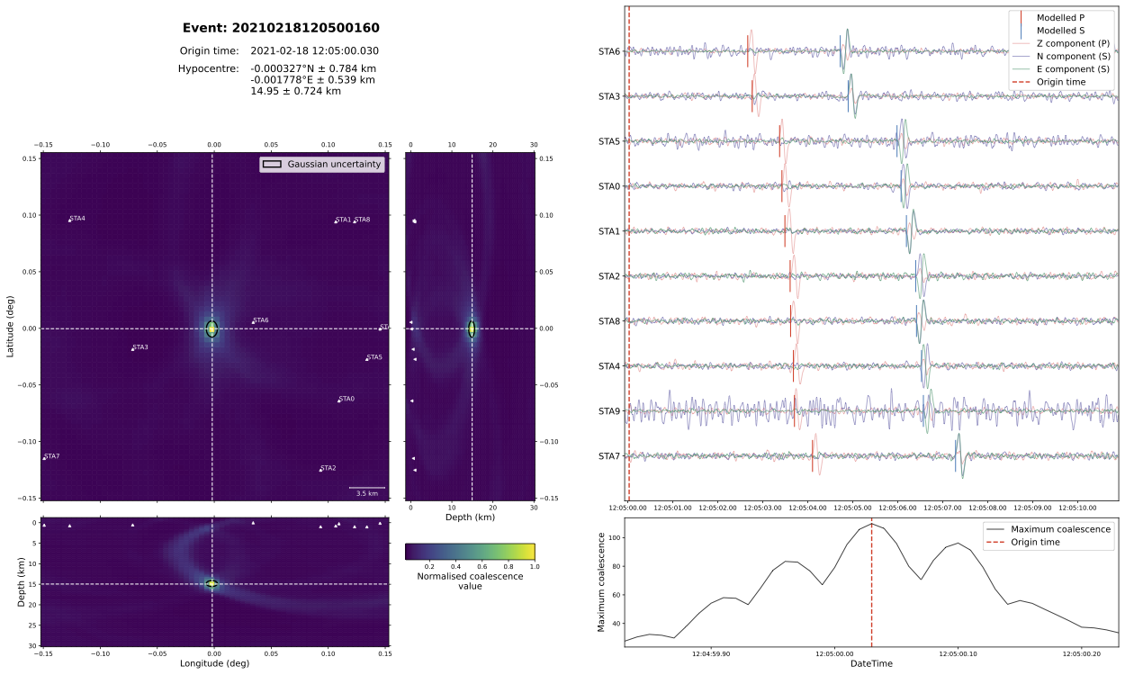
For the synthetic example, we can see in the below summary plot that we recover an earthquake location that corresponds closely with the (0.0, 0.0, 15 km) input location, and 12:05:00.0 input origin time.

../../_images/synthetic_locate_summary.png

The full script looks like this:

"""
This script runs the locate stage for the synthetic example described in the tutorial
in the online documentation.

:copyright:
    2020–2024, QuakeMigrate developers.
:license:
    GNU General Public License, Version 3
    (https://www.gnu.org/licenses/gpl-3.0.html)

"""

# Stop numpy using all available threads (these environment variables must be
# set before numpy is imported for the first time).
import os

os.environ.update(
    OMP_NUM_THREADS="1",
    OPENBLAS_NUM_THREADS="1",
    NUMEXPR_NUM_THREADS="1",
    MKL_NUM_THREADS="1",
)

from quakemigrate import QuakeScan
from quakemigrate.io import Archive, read_lut, read_stations
from quakemigrate.signal.onsets import STALTAOnset
from quakemigrate.signal.pickers import GaussianPicker


# --- i/o paths ---
station_file = "./inputs/synthetic_stations.txt"
data_in = "./inputs/mSEED"
lut_out = "./outputs/lut/example.LUT"
run_path = "./outputs/runs"
run_name = "example_run"

# --- Set time period over which to run locate ---
starttime = "2021-02-18T12:03:50.0"
endtime = "2021-02-18T12:06:10.0"

# --- Read in station file ---
stations = read_stations(station_file)

# --- Create new Archive and set path structure ---
archive = Archive(
    archive_path=data_in, stations=stations, archive_format="YEAR/JD/STATION"
)

# --- Load the LUT ---
lut = read_lut(lut_file=lut_out)

# --- Create new Onset ---
onset = STALTAOnset(position="centred", sampling_rate=100)
onset.phases = ["P", "S"]
onset.bandpass_filters = {"P": [1, 14, 2], "S": [1, 14, 2]}
onset.sta_lta_windows = {"P": [0.1, 1.5], "S": [0.1, 1.5]}

# --- Create new PhasePicker ---
picker = GaussianPicker(onset=onset)
picker.plot_picks = True

# --- Create new QuakeScan ---
scan = QuakeScan(
    archive,
    lut,
    onset=onset,
    picker=picker,
    run_path=run_path,
    run_name=run_name,
    log=True,
    loglevel="info",
)

# --- Set locate parameters ---
scan.marginal_window = 0.2
scan.threads = 4  # NOTE: increase as your system allows to increase speed!

# --- Toggle plotting options ---
scan.plot_event_summary = True

# --- Toggle writing of waveforms ---
scan.write_cut_waveforms = False

# --- Run locate ---
scan.locate(starttime=starttime, endtime=endtime)