2.1. Traveltime Lookup Tables (LUTs)
This tutorial covers the basic ideas and definitions underpinning traveltime lookup tables in QuakeMigrate, as well as demonstrating how they are made.
In order to reduce computational costs during runtime, traveltime lookup tables (LUTs) are pre-computed for each seismic phase and each station in the network to every node in a regular 3-D grid. This grid spans the volume of interest, herein termed the coalescence volume, within which QuakeMigrate will search for events.
2.1.1. Defining the underlying 3-D grid
Each traveltime LUT is defined on the same regular 3-D grid which spans the volume of interest. This grid is related to geographical space by a pair of projections that are related by some geometric transformation.
2.1.1.1. Coordinate projections
First, a pair of coordinate reference systems are defined to represent the input coordinate space (cproj) and the Cartesian grid space (gproj). This is done using pyproj, which provides the Python bindings for the PROJ library. It is important to think about which projection is best suited to your particular study region. More information can be found in their documentation.
Warning
The default unit of distance of Proj is the metre! It is strongly advised that you explicitly state which unit of distance you wish to use.
In the following example, the WGS84 reference ellipsoid (used as standard by the Global Positioning System) is used as the input space and the Lambert Conformal Conic projection is used to relate this to a Cartesian grid space:
from pyproj import Proj


cproj = Proj(
    proj="longlat", ellps="WGS84", datum"=WGS84", no_defs=True
)
gproj = Proj(
    proj="lcc",
    lon_0=116.75,
    lat_0=6.25,
    lat_1=5.9,
    lat_2=6.6,
    datum="WGS84",
    ellps="WGS84",
    units="km",
    no_defs=True,
)
The unit of distance of the Cartesian grid space is specified as kilometres. lon_0 and lat_0 specify the geographic origin of the projection (which should be at roughly the centre of your grid), and lat_1 and lat_2 specify the two “standard parallels”, which set the region in which the distortion from unit scale is minimised. It is therefore recommended that you choose latitudes at ~25% and 75% of the North-South extent of your grid (see Geographical location and spatial extent).
Note
The values used in this LCC projection are for a study region in Sabah, Borneo. Caution is advised in choosing an appropriate projection, particular if your study region is close to the poles. See the PROJ documentation for more details, and the full selection of projections available.
Note
It is possible to run QuakeMigrate with distances measured in metres if desired, as long as the user specifies this requirement when defining the grid projection and all other inputs (station elevations, grid specification, seismic phase velocities, etc) are consistently specified in metres or metres/second.
2.1.1.2. Geographical location and spatial extent
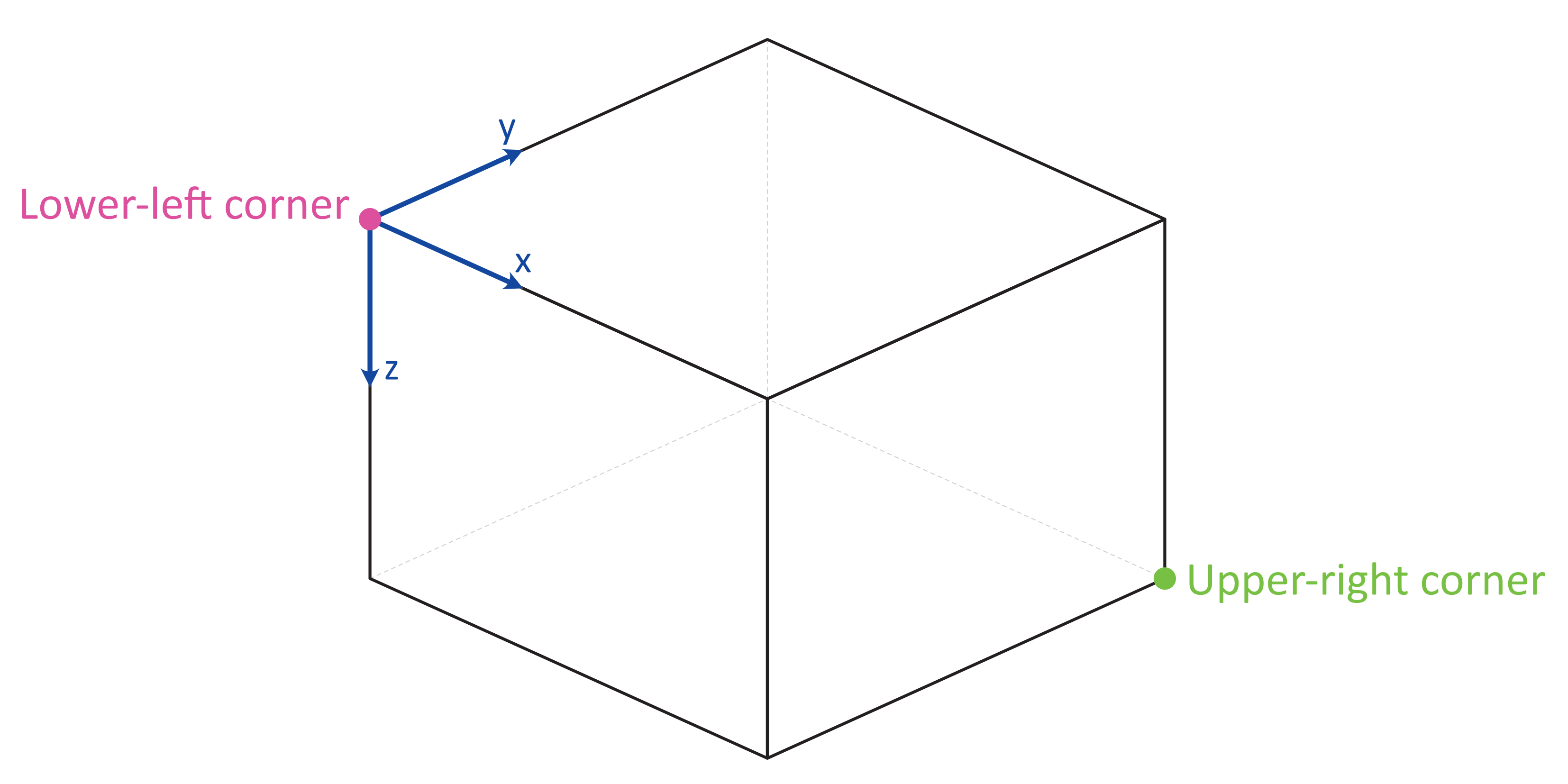
In order to geographically situate our lookup table, two reference points in the input coordinate space are specified, herein called the lower-left and upper-right corners (ll_corner and ur_corner, respectively). QuakeMigrate works in a depth-positive frame (i.e., positive-down or left-handed coordinate system); the following schematic shows the relative positioning of the two corners:
The final piece of information required to define the grid on which traveltimes will be computed is the node_spacing between grid nodes along each axis (x, y and z). The LUT class will automatically find the number of nodes required to span the specified geographical region in each dimension. If the node spacing doesn’t fit into the corresponding grid dimension an integer number of times, the location of the upper-right corner is shifted to accommodate an additional node.
ll_corner = [116.075, 5.573, -1.750]
ur_corner = [117.426, 6.925, 27.750]
node_spacing = [0.5, 0.5, 0.5]
Note
Any reduction in grid size can greatly reduce the computational cost of running QuakeMigrate, as runtime scales with the number of nodes—that is, n^3 for an equidimensional lookup table grid of side-length n. The 1-D fast-marching method for computing traveltimes requires that all stations be within the grid volume, but otherwise you are free to design the grid as you wish.
Note
The corners (ll_corner and ur_corner) are nodes. Hence a grid that is 20 x 20 x 20 km, with 2 km node spacing in each dimension, will have 11 nodes in x, y, and z.
2.1.1.3. Bundling the grid specification
The grid specification is bundled together into a dictionary to be used as an input for the compute_traveltimes() function. The AttribDict from ObsPy is used for this, which extends the standard Python dict data structure to also have .-style access.
- ::
from obspy.core import AttribDict
grid_spec = AttribDict() grid_spec.ll_corner = ll_corner grid_spec.ur_corner = ur_corner grid_spec.node_spacing = node_spacing grid_spec.grid_proj = gproj grid_spec.coord_proj = cproj
2.1.2. Computing traveltimes
2.1.2.1. Station files
In addition to the grid specification, you will need to provide a list of stations for which to compute traveltime tables.
from quakemigrate.io import read_stations


stations = read_stations("/path/to/station_file")
The read_stations() function is a passthrough for pandas.read_csv(), so we can handle any delimiting characters (e.g., by specifying read_stations("station_file", delimiter=",")). There are four required (case-sensitive) column headers - “Name”, “Longitude”, “Latitude”, “Elevation”.
Note
Station elevations are in the positive-up/right-handed coordinate frame. An elevation of 2 would correspond to 2 (km) above sea level (or, conversely, a depth of -2 (km)).
The compute_traveltimes() function used in the following sections returns a lookup table (a fully-populated instance of the LUT class) which can be used in the Detect, Trigger, and Locate stages.
A number of methods for computing traveltimes have been bundled in with QuakeMigrate, with details below.
2.1.2.2. Homogeneous velocity model
Simply calculates the straight-line traveltimes between stations and points in the grid. It is possible to use stations that are outside the specified span of the grid if desired. For example, if you are searching for basal icequakes you may limit the LUT grid to span a relatively small range of depths around the ice-bed interface.
from quakemigrate.lut import compute_traveltimes


compute_traveltimes(
    grid_spec,
    stations,
    method="homogeneous",
    phases=["P", "S"],
    vp=5.,
    vs=3.,
    log=True,
    save_file=/path/to/save_file,
)
2.1.2.3. 1-D velocity models
Similarly to station files, 1-D velocity models are read in from an (arbitrarily delimited) text file using quakemigrate.io.read_vmodel() (see below for examples). There is only 1 required (case-sensitive) column header - “Depth”, which contains the depths at the top of each layer in the velocity model. Each additional column should contain the seismic velocity for each layer corresponding to a particular seismic phase, with a (case-sensitive) header, e.g. Vp (Note: Uppercase V, lowercase phase code).
Note
The units for velocities should correspond to the units used in specifying the grid projection. km -> kms-1; m -> ms-1.
Note
Depths are in the positive-down/left-handed coordinate frame. A depth of 5 would correspond to 5 (km) below sea level.
2.1.2.3.1. 1-D fast-marching method
The fast-marching method calculates traveltimes by implicitly tracking the evolution of the wavefront. The default implementation used in QuakeMigrate is provided by the scikit-fmm package. It is possible to use this package to compute traveltimes from 1-D, 2-D, or 3-D velocity models, however currently only a utility function for computes traveltime tables from 1-D velocity models is provided. The format of this velocity model file is specified below. See the scikit-fmm documentation and Rawlinson & Sambridge (2005) for more details.
Note
Using this method, traveltime calculation can only be performed between grid nodes: the station location is therefore taken as the closest grid node. For large node spacings this may cause a modest error in the calculated traveltimes.
Note
All stations must be situated within the grid on which traveltimes are to be computed.
from quakemigrate.lut import compute_traveltimes
from quakemigrate.io import read_vmodel


vmod = read_vmodel("/path/to/vmodel_file")
compute_traveltimes(
    grid_spec,
    stations,
    method="1dfmm",
    phases=["P", "S"],
    vmod=vmod,
    log=True,
    save_file=/path/to/save_file,
)
The format of the required input velocity model file is specified above.
2.1.2.3.2. 1-D NonLinLoc Grid2Time Eikonal solver
Uses the Grid2Time Eikonal solver from NonLinLoc under the hood to generate a 2-D traveltime grid spanning the distance between a station and the point in the lookup table grid furthest away from its location. This slice is then “swept” through the necessary range of azimuths to populate the 3-D traveltime grid using a bilinear interpolation scheme. This method has the benefit of being able to include stations outside of the volume of interest, allowing the user to specify the minimum grid dimensions required to image the target region of seismicity.
Note
Requires the user to install the NonLinLoc software package (available from https://github.com/ut-beg-texnet/NonLinLoc)—see the Installation instructions for guidance.
from quakemigrate.lut import compute_traveltimes
from quakemigrate.io import read_vmodel


vmod = read_vmodel("/path/to/vmodel_file")
compute_traveltimes(
    grid_spec,
    stations,
    method="1dnlloc",
    phases=["P", "S"],
    vmod=vmod,
    block_model=False,
    log=True,
    save_file=/path/to/save_file,
)
The format of the required input velocity model file is specified above.
2.1.2.4. Other formats
It is also straightforward to import traveltime lookup tables generated by other means. A basic parser is provided for lookup tables stored in the NonLinLoc format (read_nlloc()). This code can be adapted to read any other traveltime lookup table, so long as it is stored as an array: create an instance of the LUT class with the correct projections and grid dimensions, then add the (C-ordered) traveltime arrays to the LUT.traveltimes dictionary using:
lut.traveltimes.setdefault(
    STATION,
    {},
).update(
    {PHASE.upper(): traveltime_table}
)
where STATION and PHASE are station name and seismic phase strings, respectively (e.g., ST01 and P).
2.1.3. Saving your LUT
If you provided a save_file argument to the compute_traveltimes() function, the LUT will already be saved. The pickle library (a Python standard library) is used under the hood to serialise the LUT, which essentially freezes the state of the LUT. If you did not provide a save_file argument, or have added 3rd-party traveltime lookup tables to the LUT, you will need to save it using:
lut.save("/path/to/output/lut")
In any case, the lookup table object is returned by the compute_traveltimes() function allowing you to explore the object further if you wish.
2.1.4. Reading in a saved LUT
When running the main stages of QuakeMigrate (detect(), trigger(), and locate())
it is necessary to read in the saved LUT, which can be done as:
from quakemigrate.io import read_lut


lut = read_lut(lut_file="/path/to/lut_file")
2.1.5. Decimating a LUT
You may wish to experiment with different node spacings, to find the optimal balance between computational requirements (runtime and memory usage), resolution, and detection sensitivity. The LUT object has decimation functionality built-in, e.g.:
lut = lut.decimate([2, 2, 2])
will decimate (increase the node spacing) by a factor of 2 in each of the x, y and z dimensions.
Note
The lut.decimate() function is (by default) not carried out in-place, so you need to explicitly set the variable lut equal to the returned copy. Alternatively, use inplace=True.
Note
Where the decimation factor d is not a multiple of n - 1, where n is the number of grid nodes along the given axis, one or more grid nodes will be removed from the upper-right-corner direction of the LUT, which will accordingly slightly reduce the grid extent.